The 12 Tanks Puzzle- Solved with AMR
This fluid dynamics related puzzle went viral on Facebook a few years back. I guess when Einstein taunts you it is pretty hard to resist giving it a go.
Lets use this puzzle to describe the process we go through as computational fluid dynamicists when approaching a novel problem for the first time while also showing off a recently introduced capability in Simcenter STAR-CCM+ that is unlocking a new class of industrial problems to CFD analysis.
Step 1: Use engineering judgement to make the most reasonable assumptions where information is lacking. In this case, we must assume quite a lot, for example, the gravitational constant and direction, the fluid and gas properties (water and air at standard conditions), flowrate (2.2 gpm), tank geometry (paint cans), and physical scale (1.5” Sch 40 pipe fittings) to name a few.
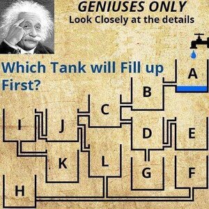
Step 2: Form a mental picture of the system dynamics using the simplest possible set of physics and conditions that will accurately assess the quantities of interest. Here our quantity of interest is simply knowing which bucket fills first. A careful inspection of the connections at tanks D and H reveals that two flow paths are blocked. This allows us to omit tanks D, E, G and H from the analysis. Once that is noticed, intuition leads most people to assume that bucket F will fill first based purely upon the concept that as the water level rises in an individual bucket it will not go any higher before first filling lower buckets to the same level. This is the most common “solution” you’ll find on the internet as well.
Step 3: Establish the computational physics models that will help you solve the problem. In this case we’ll use a transient (time-dependent), multiphase CFD approach utilizing the Volume of Fluid (VOF) methodology and with gravitational forces included. We will assume both air and water are incompressible, the flow is turbulent and use a segregated solver approach.
Step 4: Perform a simulation on a coarse computational grid to establish precedence at the lowest time and effort. An animation of the simulation on a fairly coarse-grid with approximately 100,000 cell volumes is shown below.
The result looks a bit strange and nonphysical so we have to ask ourselves, “What is going on here?”. An important quality of a system of immiscible fluids (air and water, in this example) is that these fluid phases always remain separated by a sharp interface. In our coarse grid simulation it looks like this phase interface is getting smeared, for the lack of a better word. To understand what is going on we first acknowledge that the VOF method is a submodel within an Eulerian Multiphase CFD model where at each computational cell the volume fraction of individual fluid phases are solved and assigned a value between 0 and 1. Now, imagine a droplet within a computational cell that is larger than the droplet itself. The computational solver has no choice but to assign that cell a liquid volume fraction not 1 or 0, as would be the case if the cell were clearly inside or outside of the fluid/gas interface, but some intermediary value representing the average volume fraction within the entire cell volume. This partial volume fraction is then subject to be convected away from the interface in this liquid/gas mixture according to the Navier-Stokes and continuity equations. A much finer grid is needed near the interface in order to keep these phases separate and prevent this nonphysical numerical diffusion.
The 12 Tanks puzzle is a prime example of why it has been difficult to accomplish this in the past. We don’t know, a priori, where the fluid interface will be throughout the duration of the simulation and so do not know where to concentrate our cell size refinements. And specifying a highly refined grid, such as that needed to resolve a fluid interface, over the entire domain is computationally expensive and inefficient. We have, in the past, had to give up on some free-surface flow projects due to the time required for the computational solver on such very fine grids.
The result looks a bit strange and nonphysical so we have to ask ourselves, “What is going on here?”.
Thankfully, in February of this year Siemens released Simcenter STAR-CCM+ 2020.1 which includes an Adaptive Mesh Refinement (AMR) technology that alleviates this pain point. AMR (not to be confused with ASMR as mentioned in our previous post) is a dynamic method that refines or coarsens cells based on adaptive mesh criteria as the model queries the flow solution periodic intervals. Solution quantities are automatically interpolated to the newly adapted mesh. Simcenter STAR-CCM+ supports two types of adaptive mesh criteria; 1) a user-defined mesh adaptation strategy where the user provides a field function or a table that prescribes how the AMR solver is to drive mesh adaptation and 2) a model-driven mesh adaptation strategy where the adaptation criteria are provided automatically from the Simcenter STAR-CCM+ models.
In this case we use the model-driven AMR strategy for free-surface interface capturing which, as one would assume, refines the mesh in the proximity of the free surface with the goal of maintaining a sharp interface. Other built-in model-driven strategies include those for overset meshing / moving bodies and for reacting flows.
To get a feel for the implementation take a look at the following. The graphic in the lower right of the animation demonstrates how the mesh is being updated as the free surface interface is evolving. Our model size increases from 100,000 to a maximum of around 800,000 cell volumes over the course of the simulation, but this is still orders of magnitude lower than would be needed if a highly refined mesh were needed throughout the domain. The result is a much more physically intuitive and accurate simulation. Play the animation and see for yourself whether your intuition is confirmed.
Surprise! Because of the increasing pipe losses (flow resistances) in the system as each successive tank fills and flows to the next, the top most tank (A) cannot drain faster than it is being filled. Though one might argue that Tank B saw some splashing that reached the top of the tank first, it is clear that tank A is the first to fully overflow under these conditions which is our interpretation of the correct solution to the problem statement. This is why we love CFD, discovering the unexpected where all other types of analyses fall short!